
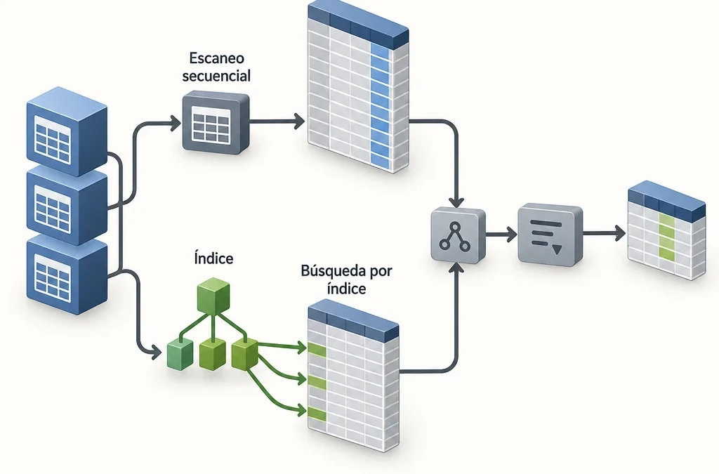
When an Odoo view takes eight seconds to load or a report ties up the administration team, it’s tempting to create an index and wait. To reliably optimize queries in PostgreSQL, you need to follow a different process: identify the query that’s causing the most lag, review its execution plan, choose the appropriate index, and measure the performance before and after.
We’ll continue this overview with a typical Odoo query, from index detection to index validation. We’ll also examine the cost of that index in terms of write operations and maintenance, because the goal is to improve the overall performance of the business, not to achieve an index scan at any cost.
Key points:
- Prioritize by total time in pg_stat_statements, not by the slowest query.
- The cost of the plan is expressed in arbitrary units, not in milliseconds.
- A Seq Scan is suitable for small tables or bulk reads.
- EXPLAIN ANALYZE executes the statement: it protects the UPDATE and DELETE statements with a transaction.
- Each new index increases the cost of INSERT, UPDATE, DELETE, and VACUUM operations.
- Validate using multiple runs, a controlled cache, and a real-world data volume.
Which queries should be optimized first?

Start with the queries that account for the most total execution time, not the slowest one on its own. A 40-millisecond query that runs 200,000 times a day consumes about 8,000 seconds, while a 30-second report run twice adds up to only 60. The pg_stat_statements extension gives you that big-picture view.
Enable pg_stat_statements
The extension is part of the PostgreSQL contrib modules and must be loaded when the server starts. In a deployment with Docker, add `shared_preload_libraries = 'pg_stat_statements'` to the `postgresql.conf` file mounted in the container, or pass that setting using the `-c` option in the service command. Then restart the container and run `CREATE EXTENSION pg_stat_statements;` in the Odoo database.
Keep in mind that the change requires restarting PostgreSQL, so it's best to schedule it outside of business hours. The extension's overhead is low and is more than offset by the insights it provides.
Sort by actual impact
To see how much each query contributes to the load, sort by `total_exec_time` rather than just by `mean_exec_time`:
```sql```
SELECT statements,
round(total_exec_time::numeric, 0) AS total_ms,
round(mean_exec_time::numeric, 1) AS average_ms,
rows,
shared_blks_hit, shared_blks_read,
left(query, 120) AS query
FROM pg_stat_statements
ORDER BY total_exec_time DESC
LIMIT 10;
```
The ratio of `shared_blks_hit` to `shared_blks_read` indicates how much data is served from the PostgreSQL cache and how much requires a read from disk or the operating system cache. A query with many blocks read and few rows returned is a clear candidate to benefit from an index.
As an example, imagine that the query launched by Odoo's ORM when opening a customer's invoice list appears in the first position. It takes an average of 180 ms and runs 45,000 times a day, which adds up to about 8,100 seconds daily—more than two hours of CPU time. That is the query we’ll be focusing on for the rest of this article.
How does Odoo's ORM generate these queries?
The ORM translates every `search()`, `read_group()`, or list view into SQL with a very recognizable pattern. If you know how to read it, you'll know which index is missing without touching any Python code. In our example, `pg_stat_statements` shows something like this, with the parameters normalized:
```sql```
SELECT "account_move"."id" FROM "account_move"
WHERE ("account_move"."company_id" IN ($1))
AND ("account_move"."move_type" IN ($2, $3))
AND ("account_move"."state" = $4)
AND ("account_move"."partner_id" = $5)
ORDER BY "account_move"."invoice_date" DESC, "account_move"."id" DESC
LIMIT 80;
```
There are several typical features. The filter by `company_id` appears due to the multi-company rules, even if you only have one company. The `ORDER BY` comes from the model’s `_order` or the view, and the `LIMIT 80` corresponds to the default pagination of the list view. The ORM then issues a second query to retrieve the visible fields for those 80 identifiers.
Each field declared with `index=True` in the model generates a single-column B-tree index. In `account_move`, `partner_id` and `state` are usually indexed separately. The planner can use one, but with separate indexes, it doesn’t handle filtering and sorting simultaneously very well. That’s why some execution plans end up reading thousands of rows just to return 80.
Before making any changes, also check whether the slowness is caused by a field calculated with `store=False` or by a complex indexing rule. No index can fix a rule that generates subqueries on `res_partner` for every row.
How to Read an Execution Plan Using EXPLAIN


A plan is a node tree: children produce rows, and parents consume them. It is read from the inside out. For each node, it compares the estimated rows with the actual ones and identifies where time is concentrated and where the largest number of blocks are read.
EXPLAIN vs. EXPLAIN (ANALYZE, BUFFERS)
`EXPLAIN` on its own displays the estimated execution plan without actually executing anything. It is based on table statistics and is instantaneous, but it only provides estimates. `EXPLAIN (ANALYZE, BUFFERS)` actually executes the query and adds real execution times, actual rows per node, and blocks read from the cache (`shared hit`) or from outside the cache (`read`).
Remember that ANALYZE executes the statement. An `EXPLAIN ANALYZE DELETE` deletes rows, and an `UPDATE` modifies data and triggers triggers. To analyze write operations, always include them in a transaction like this:
```sql```
BEGIN;
EXPLAIN (ANALYZE, BUFFERS) UPDATE account_move SET . WHERE .;
ROLLBACK;
```
Even with ROLLBACK, the statement acquires locks while it is executing. Therefore, to analyze a production statement, it is best to use a copy restored from the most recent backup.
Cost, rows, and blocks
A typical node looks like this:
```
Index Scan using the account_move_partner_id_index on the account_move table
(cost=0.43.9821.55 rows=310 width=8)
(current time=0.05.171.20 rows=4120 loops=1)
Filter: (state = 'posted' AND move_type = ANY (.))
Rows Removed by Filter: 2,950
Buffers: shared hits=1,210, reads=5,340
```
The cost (`0.43.9821.55`) is expressed in the planner's arbitrary units. The two values indicate the initial and total costs in relative terms; they are not equivalent to milliseconds. They are used to compare alternative plans for the same query, not to predict execution times. The actual time is in `actual time`.
Look for three signs. The first is that 310 rows were estimated, but 4,120 were returned—more than 13 times the expected number—which usually indicates inaccurate statistics. The second is that `Rows Removed by Filter` shows that the index locates rows that are then discarded. The third is that the 5,340 blocks read from outside the cache, at 8 kB per block, amount to about 42 MB of read operations to return 80 identifiers.
Above this node, a `Sort` operation will be performed on the 4,120 rows to apply the `ORDER BY invoice_date DESC` before the `LIMIT`. That's where the entire bottleneck lies: locating too many rows, filtering them, and sorting them in memory.
For long queries, export the query using `FORMAT JSON` and paste it into explain.dalibo.com, which renders the tree and highlights the most expensive nodes. If you’re using PostgreSQL 18, released on September 25, 2025, EXPLAIN also shows more details on I/O, index searches, and WAL activity per node, which speeds up this diagnosis.
Is sequential scanning always a problem?

No. A Seq Scan is the best option when the table is small or the query needs a large portion of its rows. Reading pages in order is much more efficient than jumping randomly between the index and the table.
The planner chooses from among four main strategies:
- Seq Scan: Scans the entire table. It is suitable for tables with a few thousand rows, such as `res_company` or `account_journal`, and for reports that aggregate nearly all the data.
- Index Scan: Scans the index and accesses the table (the heap) for each row found. It is ideal for a small number of rows or for returning them already sorted.
- Bitmap Heap Scan: First, it builds a map of the pages containing valid rows, and then reads them in physical order. It is suitable for intermediate-sized ranges, from hundreds to tens of thousands of rows, and can combine multiple indexes using `BitmapAnd`.
- Index-Only Scan: Returns results using only the index, without accessing the table, provided that the visibility map is up to date. This is the most efficient method.
A Seq Scan is indeed a sign of a problem when it occurs on `account_move_line`, `stock_move`, or `mail_message`—tables with millions of rows—and returns only a few dozen rows. In that case, a value for `Rows Removed by Filter` close to the total number of rows in the table gives it away.
You should also avoid forcing the use of an index with `SET enable_seqscan = off`, except as a one-time experiment in a session. This is useful for seeing what cost the planner would estimate with the index, but it should never be left as a permanent setting.
Why PostgreSQL Ignores an Existing Index
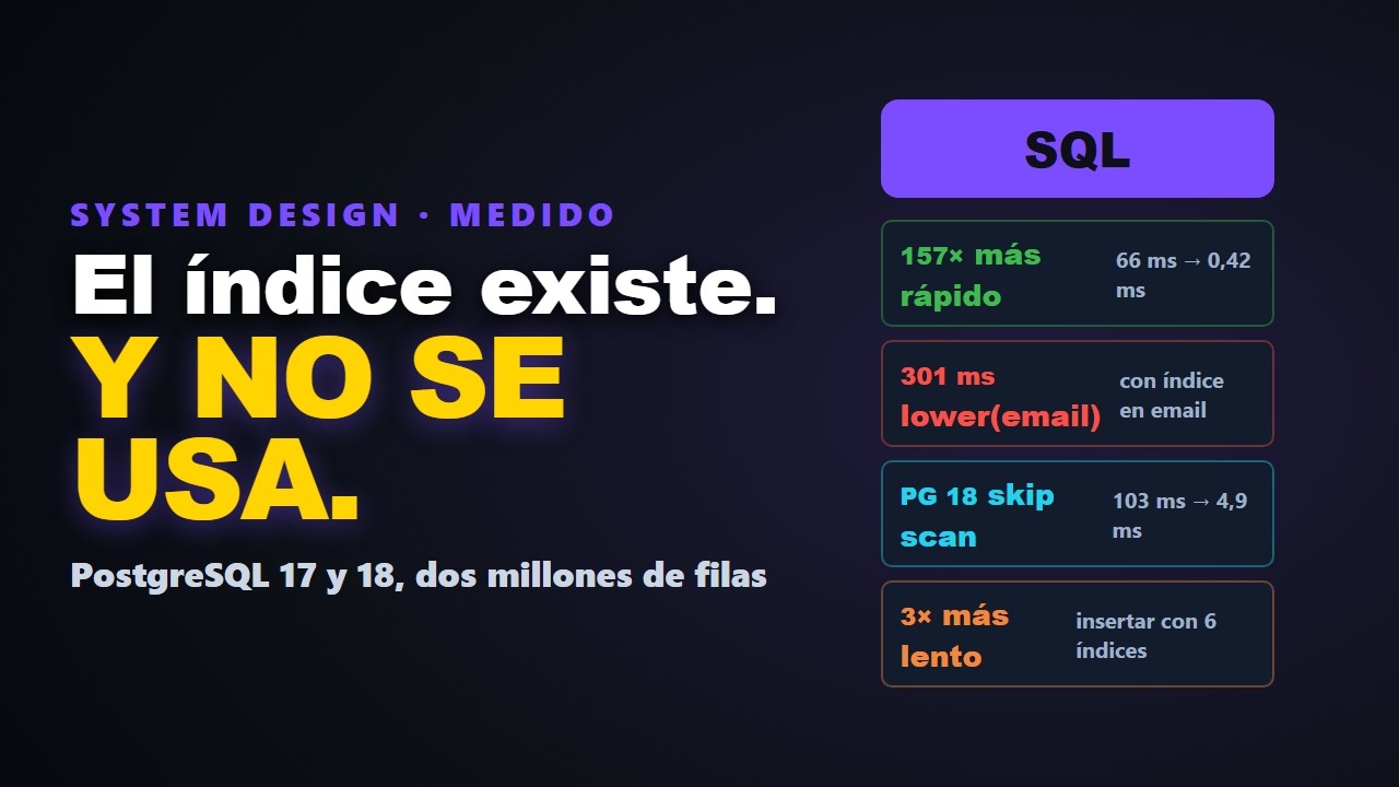
The planner ignores an index when it determines that another route is cheaper. Common causes include outdated statistics, a condition that prevents the index from being used, or such low selectivity that it is more cost-effective to read the entire table.
Statistics, ANALYZE, and autovacuum
All row estimates are derived from the statistics collected by `ANALYZE`: most frequent values, histograms, and the proportion of nulls per column. If, after a bulk import or data migration, those statistics still describe the table as it was before, the planner will make the wrong choice. Run `ANALYZE account_move;` after any large data load.
Autovacuum automatically runs ANALYZE when approximately 10% of the rows have changed (`autovacuum_analyze_scale_factor = 0.1`) and VACUUM when approximately 20% have changed. For tables with 20 million rows, that means waiting for 2 million changes. For large Odoo tables, lower these thresholds for each table:
```sql```
ALTER TABLE account_move_line
SET (autovacuum_analyze_scale_factor = 0.02,
autovacuum_vacuum_scale_factor = 0.05);
```
VACUUM is also important for the execution plan. It maintains the visibility map that enables Index-Only Scans and removes dead tuples, which bloat tables and indexes. Check `n_dead_tup` and `last_autoanalyze` in `pg_stat_user_tables` to verify that maintenance is performed on time. If a column has a very skewed distribution—such as `state`, where 95% of the values are `posted`—increase the sample size with `ALTER TABLE . ALTER COLUMN state SET STATISTICS 1000;`.
Conditions That Prevent You From Taking Advantage of the Index
A B-tree index on `name` is not suitable for `WHERE lower(name) = .`, nor for `ILIKE '%text%'`, nor when there is an implicit type conversion. Odoo generates many `ILIKE` queries on name fields. For those queries, the appropriate index is a GIN index with `pg_trgm`, which Odoo creates for fields declared with `index='trigram'`.
In a composite index, the order of the columns also matters. An index `(company_id, partner_id)` is of little help to a query that filters only by `partner_id`. PostgreSQL 18 added the B-tree skip scan, which in some cases can utilize indexes without using their first column, but it is only effective when that column has few distinct values.
How to Design a B-Tree, Compound, or Partial Index
For our invoice query, the right choice is a composite, partial B-tree index that covers both the filter's equality conditions and the sort order of the results. This way, PostgreSQL reads only the first 80 entries and does not sort anything in memory.
The order of columns in a composite index
First, place the columns filtered by equality, then those by range, and finally the `ORDER BY` columns in the same order. Among the equality columns, start with the one you use most often on its own in other queries, because the index works for any prefix of its columns. The PostgreSQL documentation illustrates this concept with a `(major, minor)` index for queries that filter by both.
In this example, `partner_id` comes first (it filters by equality and is very selective), followed by `invoice_date DESC` and `id DESC` for sorting:
```sql```
CREATE INDEX CONCURRENTLY account_move_partner_invoice_idx
ON account_move (partner_id, invoice_date DESC, id DESC)
WHERE state = 'posted'
AND move_type IN ('out_invoice', 'out_refund');
```
`company_id` is omitted because, with only one company, it doesn't filter anything. If you're working with multiple companies and the data is actually separated by company, add it right after `partner_id`.
When to Choose a Partial Index
A partial index stores only the rows that satisfy its `WHERE` condition. This is useful when the query always filters by the same value and that subset represents a well-defined portion of the table. If drafts, journal entries, and vendor invoices account for 60% of `account_move`, the index occupies less than half of the table. Furthermore, transactions involving those excluded rows do not modify the index.
The planner only uses it if the query logically implies its condition. If the ORM sends `state = $4` as a generic parameter, it may not recognize that implication in generic plans. It checks that the index appears in the final plan and uses `CONCURRENTLY` to avoid blocking writes while it is being built.
The cost of title deeds and maintenance
Each index is updated with every INSERT and DELETE, and with every UPDATE that affects its columns or that cannot be resolved as a HOT update. In `account_move`, confirming an invoice changes `state`, which forces the entry to be inserted into the partial index. This also increases the amount of WAL generated, the size of backups, and the workload for VACUUM.
A composite index with three columns on 3 million rows can take up approximately 100 to 150 MB. If you add it without removing anything, the shared memory ends up being distributed among more structures. Check `pg_stat_user_indexes` and drop indexes with `idx_scan = 0` after several weeks of normal activity, except for those that ensure uniqueness.
Measure Before and After Without Cheating
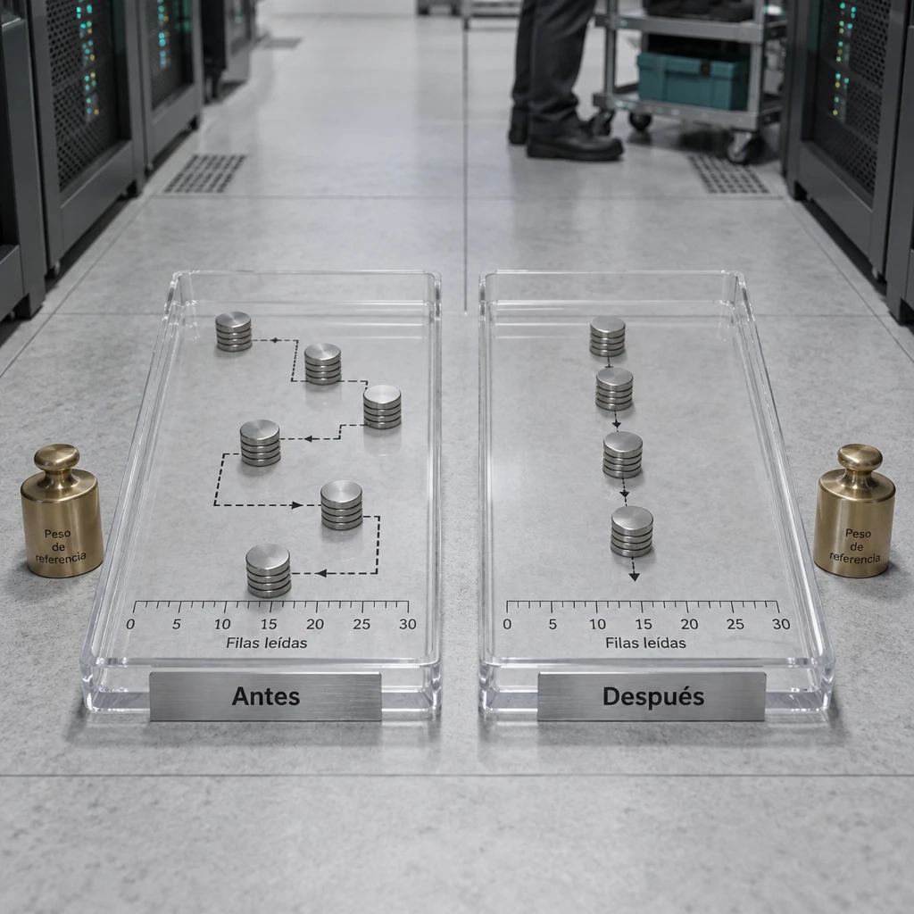
Validate each index using a reproducible measurement of the entire load, not a single run. The second run of any query is usually faster because the blocks are already in the cache. If you don't take this into account, you'll attribute an improvement to the index that isn't actually due to it.
Follow these steps:
- Restore a recent production backup to an equivalent environment—with the same amount of data and the same version of PostgreSQL—and run `ANALYZE`.
- Run the query five to ten times with `EXPLAIN (ANALYZE, BUFFERS)`, using real parameters: one customer with 20 invoices and another with 30,000. Record the median and the number of blocks read, not the best time.
- It also measures the affected writes—for example, using `pgbench` and a script that inserts and confirms invoices—and records the transactions per second and the WAL generated.
- Create the index, repeat steps 2 and 3 under the same conditions, and compare the results.
- In production, run `SELECT pg_stat_statements_reset();` after deploying the index, and after one week, compare the `total_exec_time` of the top queries with that of the previous week.
In the example, the new plan should show an Index Scan that stops after reaching 80 rows, with no Sort node and only a few dozen blocks read, compared to the previous 6,500-plus. If the median time drops from 180 ms to about 2 ms, the total time for the 45,000 daily calls decreases from about 8,100 seconds to 90.
These savings are compared with the measurements from Step 3. If invoice confirmation results in a 2% drop in performance, the net result is clearly positive. If a nightly import of 500,000 lines takes an extra hour, it might be best to disable the process and rebuild the index later. The decision is made taking into account the company’s overall workload.
Where to Start
Enable `pg_stat_statements` this week and let it collect seven days of normal activity. That list, sorted by total time, will allow you to identify the three or four queries worth optimizing and discard the rest without creating indexes blindly. If you'd prefer to have technical support for your Odoo Installation in Barcelona, Synergia offers it with a two-hour response SLA.
Frequently Asked Questions
How many indexes can a table have without affecting performance?
There is no fixed number. The limit is determined by the ratio of reads to writes. In tables with many writes, such as `account_move_line` or `stock_move`, each additional index affects the commit time, so justify each one with a specific query from `pg_stat_statements`.
Can you create an index in production without stopping Odoo?
Yes, with `CREATE INDEX CONCURRENTLY`, which does not block writes. It takes longer and cannot be executed within a transaction. If it fails, it leaves an index marked as invalid that you must drop before retrying.
How often should you run ANALYZE manually?
Autovacuum is usually sufficient, configured on a per-table basis for larger tables. Run `ANALYZE` manually after bulk imports, migrations, or large-volume deletions, because otherwise the query planner would use statistics that describe a different table.
Does increasing `work_mem` help speed up queries?
This is helpful when the plan shows sort operations or hash operations that exceed memory capacity and are offloaded to disk (`Sort Method: external merge`). Use this feature with caution: it is reserved per operation and per connection, and with many Odoo work processes, it can exhaust the server's memory.